The platform
This is the long version. The drillhole files arrive, the deposit appears, the samples are composited and domained, the variography is fitted, the block model is built and kriged, and the method that did all of it is written down as it happens. Below is each stage, with real captures of the running application. If you only want to know what ships today and what does not, that is on the proof page.
Module 01 · Data
Most of the delay in an estimation is not the geostatistics. It is getting the drillholes in — the right projection, the right dip convention, the grades on the right column — and then finding somewhere to actually look at the orebody. That is the first module's whole job, and it is where the geology either becomes visible or stays in a folder.
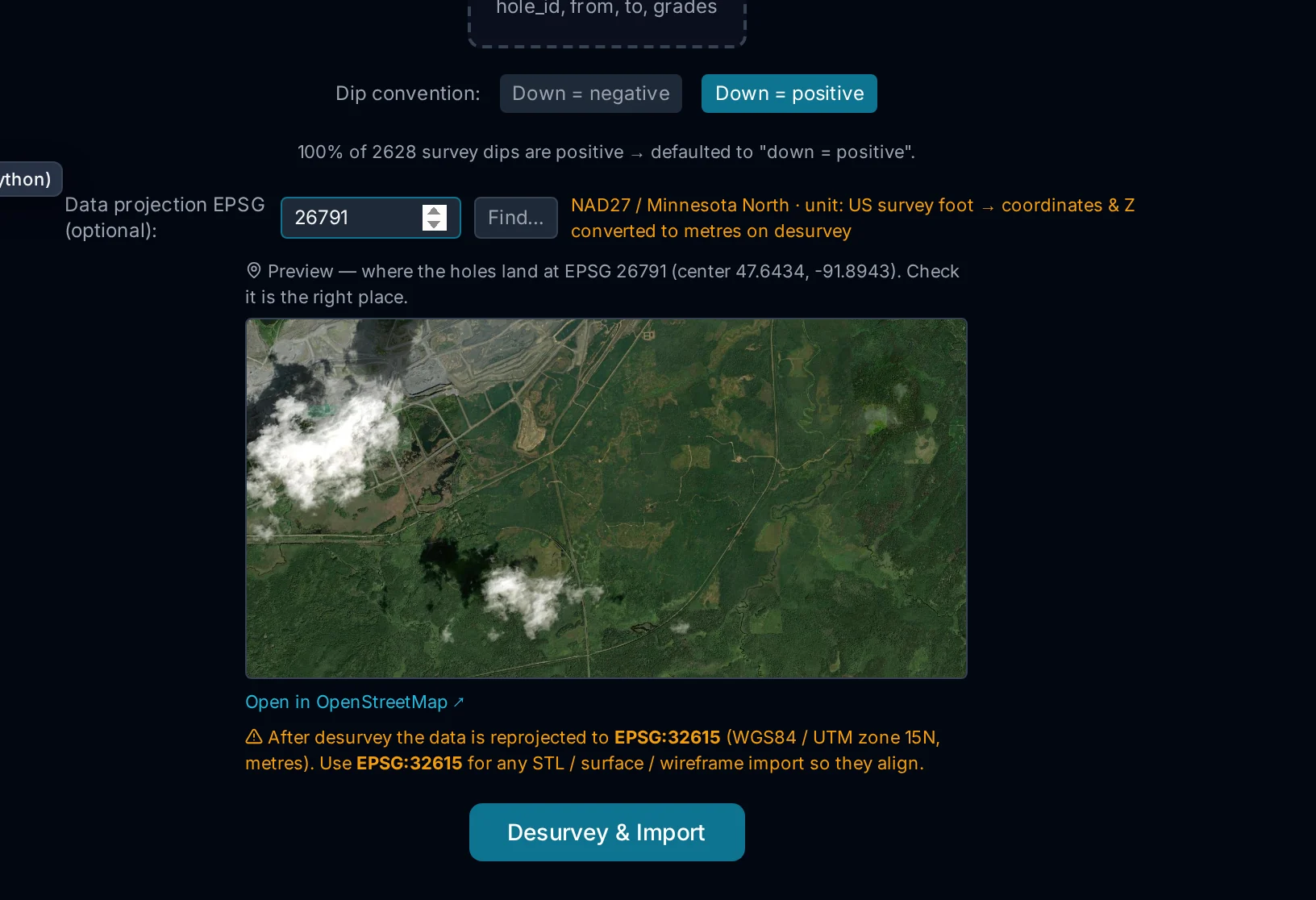
Drop three files and they sort themselves into collar, survey and assay by name. Type the source EPSG and the app tells you it is NAD27 Minnesota North in US survey feet, converts the coordinates to metres, and drops a satellite image of where your holes actually land. A projection mistake is caught in the first thirty seconds instead of in the block model.
On this trio it also reports: 100 % of 2,628 survey dips are positive → defaulted to "down = positive". It asks when it is unsure and states its assumption when it is not.
Point it at a Datamine study and it reads the
.dm
headers and tells you what each file is: drillholes, collar, survey, block
model, wireframe, variogram, variogram model, search and estimation parameters,
strings. Fields and record counts, before you import anything. You do not have to open
Datamine to know what is in the folder.
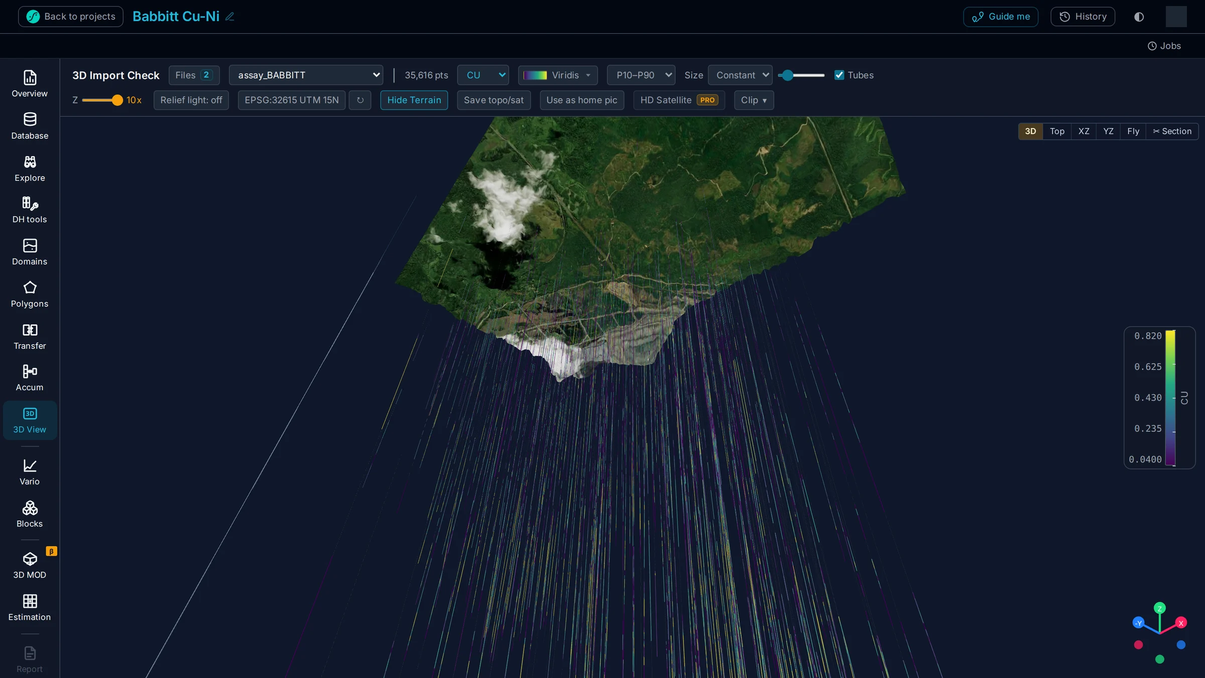
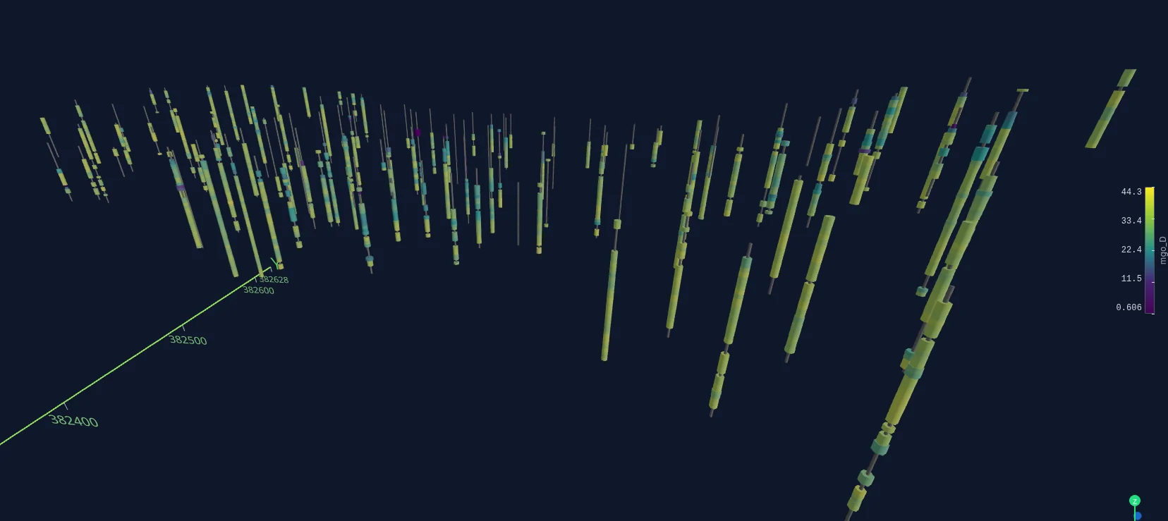
Drillholes as tubes coloured and sized by grade, wireframes and DXF surfaces in the same scene, clipping planes, a section flythrough, and the search cone drawn among the samples it actually selected. The parameters sit in the ground with the geology, not in a legend beside it.
Type the EPSG. The topography and the imagery for your licence area arrive on their own. No GIS request, no basemap licence, no waiting on another office, no cost.
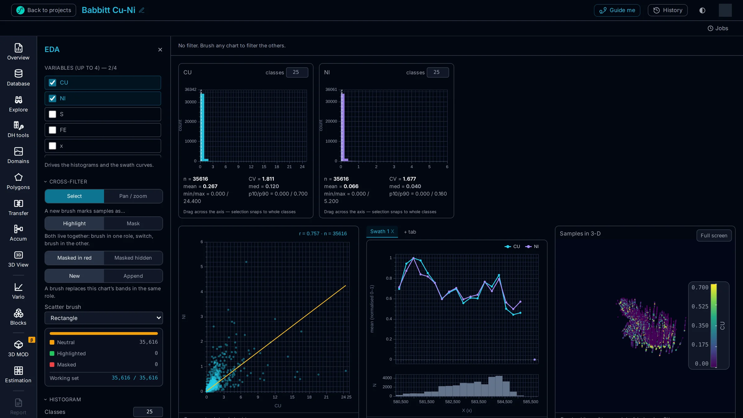
Four variables at once — grades, deleterious elements, geometallurgical responses, logged lithology — as histograms, scatter and swath, all cross-filtered, with a mini-3D beside them so a selection in a histogram is a selection in the ground. The table is virtualised, carries per-column statistics, and edits persist into the project. Looking at the geology stops being a separate exercise from modelling it.
The unglamorous half
Between the drillhole file and the estimate sits the work that never appears in the technical report: regularising the samples, throwing out the collar that was logged twice, deciding what counts as a domain, drawing the orebody, and building the grid to put it in. It is most of the elapsed time on a resource estimate, and in most companies it is spread across three packages and a spreadsheet. Here it is one continuous set of tools over one project.
Composite to a fixed support, with a mass-balance report that tells you what the regularisation cost you. Remove duplicated samples and collars. Create a variable. Aggregate to the hole head, or push a collar value back down the samples. Clip against a surface, or select on a bench polygon.
Build domains from rules on any variable — lithology, alteration, weathering profile, a grade threshold — or let the grade shell take the longest mineralised run in each hole and hand you a first pass in one click. The automatic answer is an editable starting point for a geologist, never a boundary you have to accept.
Contour a domain in plan. Build a 2.5 D sheet from a centreline and a thickness, with the border continuing the local dip instead of flattening to the mean. Or model the domain in three dimensions — morphological closing with stratigraphic flattening and a Wendland C2 interpolation — so a folded orebody is modelled in its own frame rather than in the one the survey happened to use. Stack the surfaces into a deposit model, and export any of it as DXF.
Marked honestly: live means it is in the product, next means the engine exists and is covered by the same test suite as the rest but is not yet open to every account. The chain further down draws the same line.
Module 02 · VarioForge
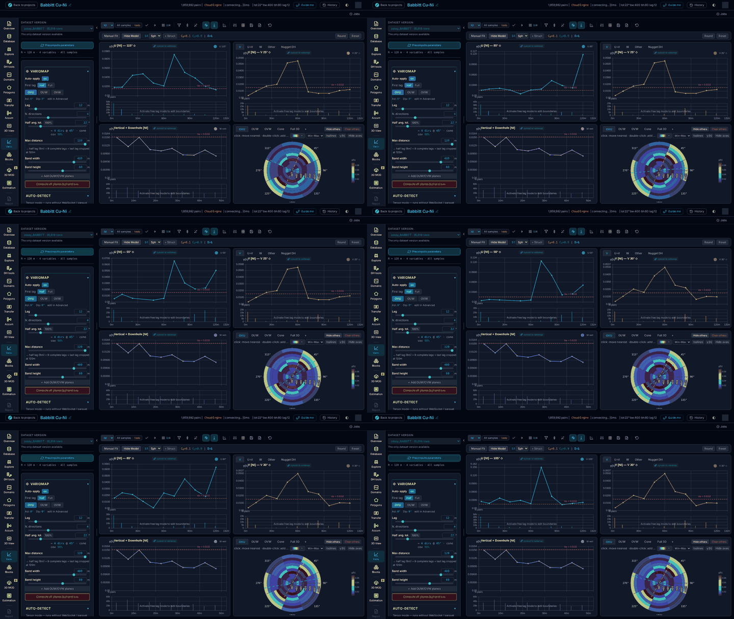
Underneath VarioForge is a calculation tree rather than a recompute. Move the azimuth, the tolerance, the bandwidth, the lag, the grade or the domain and the curve is already redrawn. It behaves the same on three hundred samples and on a full drilling campaign, and on any variable you point it at — grade, deleterious element or geometallurgical response. That is why an estimation stops being a budget of minutes per test.
When a variogram costs nothing to ask for, the question changes. It stops being "which variogram do we have time to fit" and becomes "which reading of this orebody survives". Chain a domain against a variable, look, change the domain, look again. Four grades against three domains is an afternoon, not a fortnight — so the geologist tests the interpretation they would otherwise have had to assume.
Geology, not charts
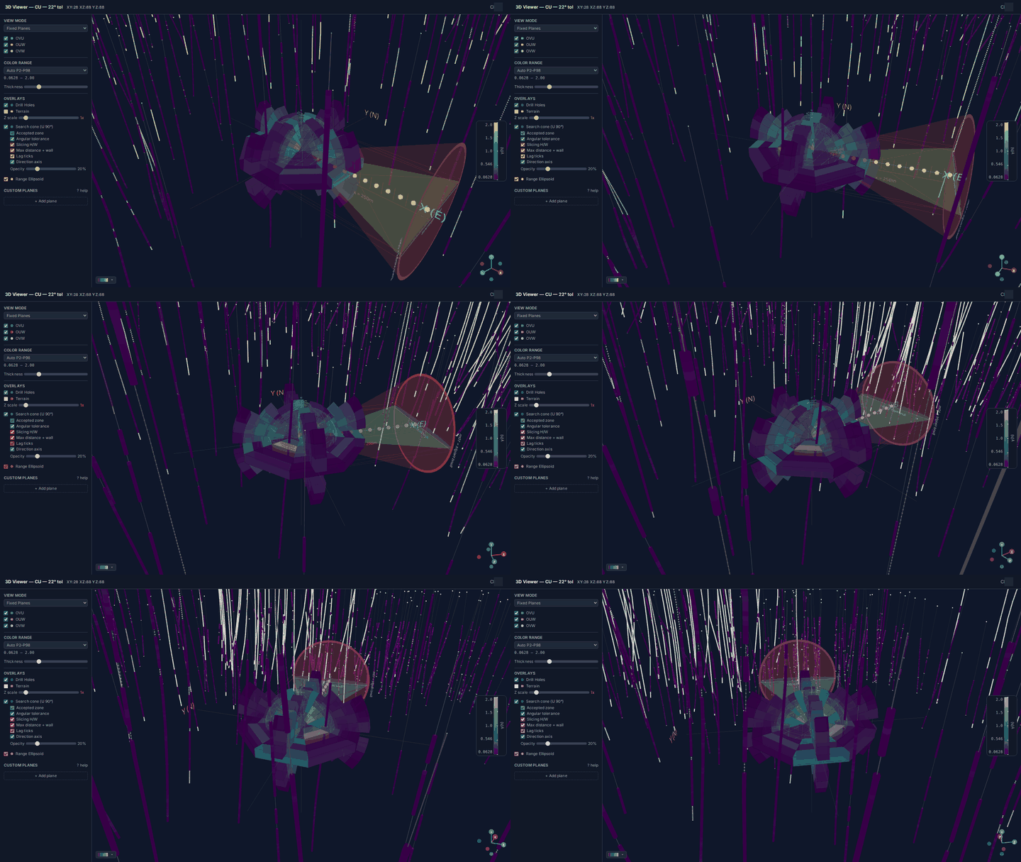
Most packages draw the result in 3D. Drawing the parameters in 3D, the cone that accepted the pairs, on the holes that produced them, is what turns a review meeting from an argument about numbers into a conversation about geology.
Build the block model inside the wireframe, sub-block it, set the search neighbourhood and run ordinary kriging on the structures the variography just produced. The same fitted model, not a set of numbers retyped into another package — for every variable the mine needs estimated, not only the payable one.
The experimental variogram, the four model types and the kriging system are asserted against independent reference implementations on every release, rotated anisotropy included. Ask for the test suite during a technical review and we hand it over.
The block model rendered inside the DXF volume it was constrained by, blocks sized and coloured by grade, turning in the same scene as the holes. Assembling the deliverable and reviewing it are the same act.
opening progressively
Module 03 · WorkflowCanvas
This is the part people do not expect. OreFrame does not only read your packages' files. It writes their work. Assemble the routine from templates on the canvas and it emits the macros and scripts those packages run, in their own syntax, then executes them in order and tells you where it is. The reasoning about the orebody moves out of one person's head and into a graph the whole mine can read — the annual resource estimate, but also grade control and the monthly production reconciliation that follow it.
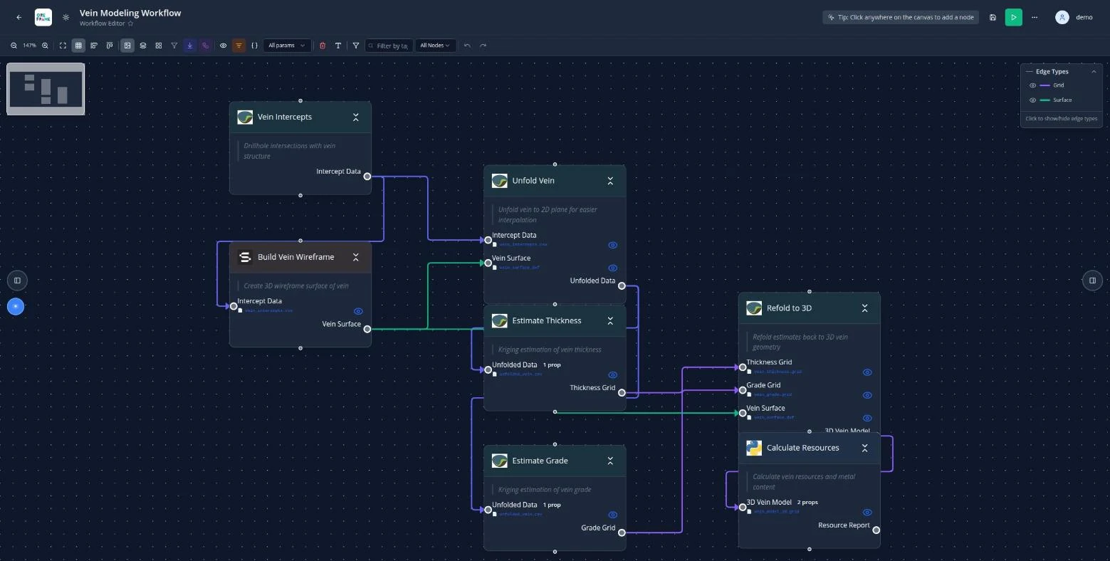
A routine can cross five packages in one run: database to QGIS to Python to Isatis to Leapfrog and back, with conditional branches driven by global variables, so the simulation runs only when the flag is set. Progress is tracked node by node and the run history is kept — which is what makes a routine safe to re-run every month against fresh production data rather than rebuilt each time.
234 for Surpac, 100 for Datamine, 90 for RMSP, 69 for Isatis, plus Python and QGIS, across block modelling, estimation, variography, compositing, DTM, blasting and underground design.
libraries live · browser being finished
Ready-made routines for nickel laterite with weathering-profile domains and moisture and density, orogenic gold with indicator kriging and heavy top-cutting, porphyry copper with alteration zones and net smelter return, and BIF iron with Davis Tube recovery and product classification. Open one, change what your orebody does differently.
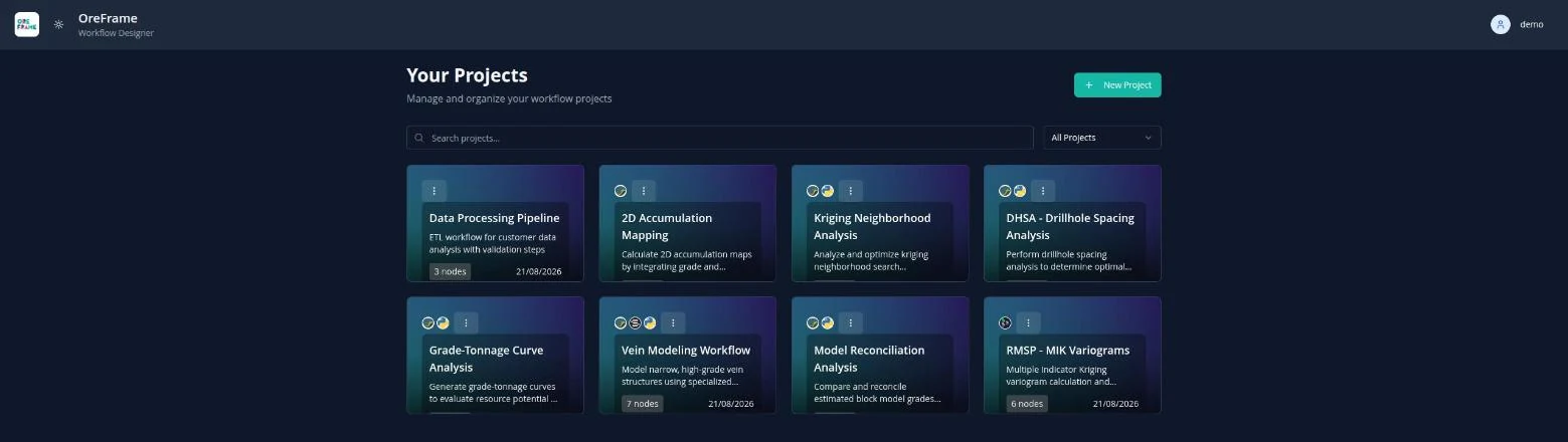
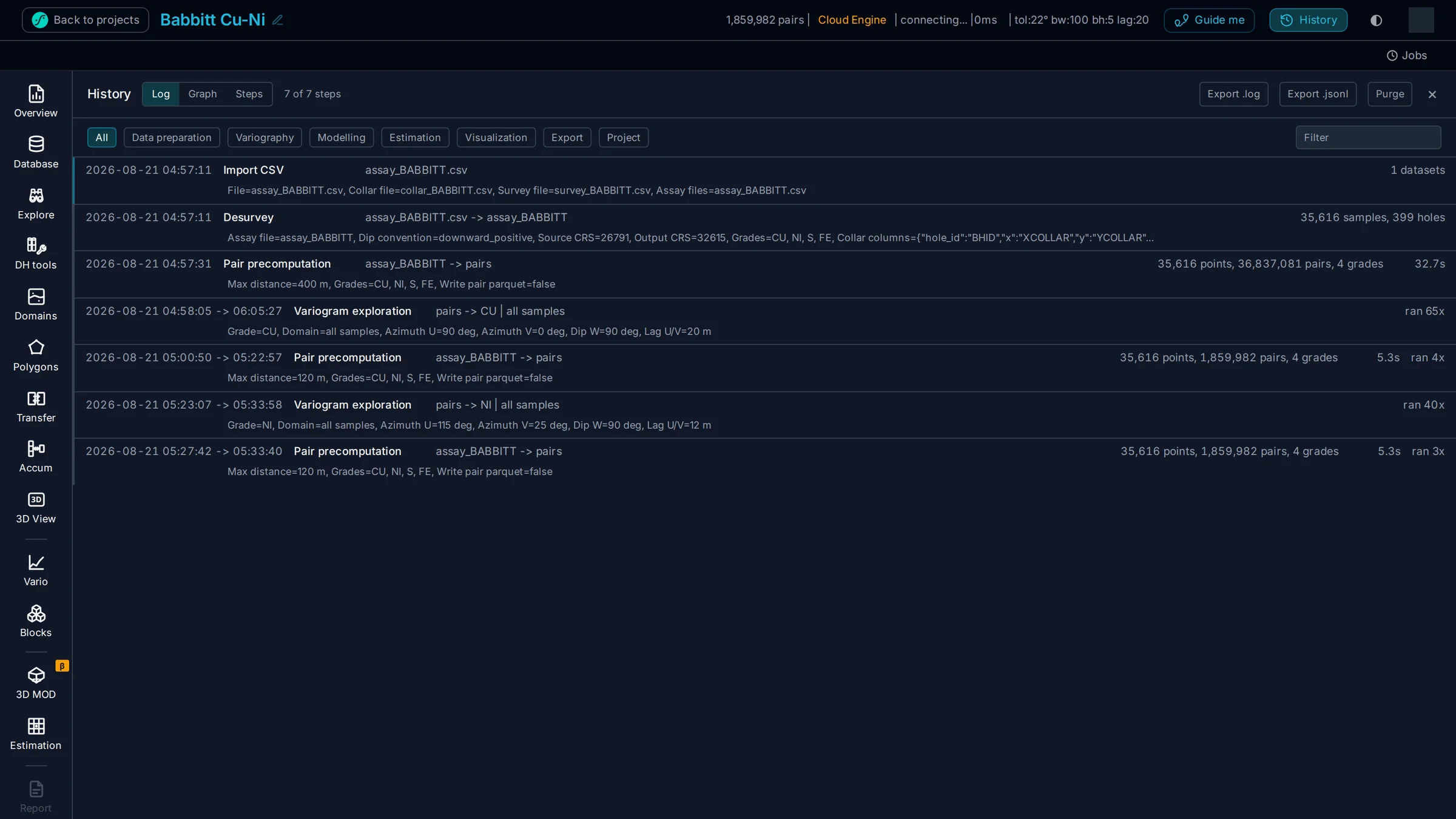
Every action in the study is recorded as a node: the import mapping, the composite length, the domain rule, the fitted structure, the search ellipsoid. Not a log file beside the model. The graph is the model's provenance, and it is the same object the canvas opens.
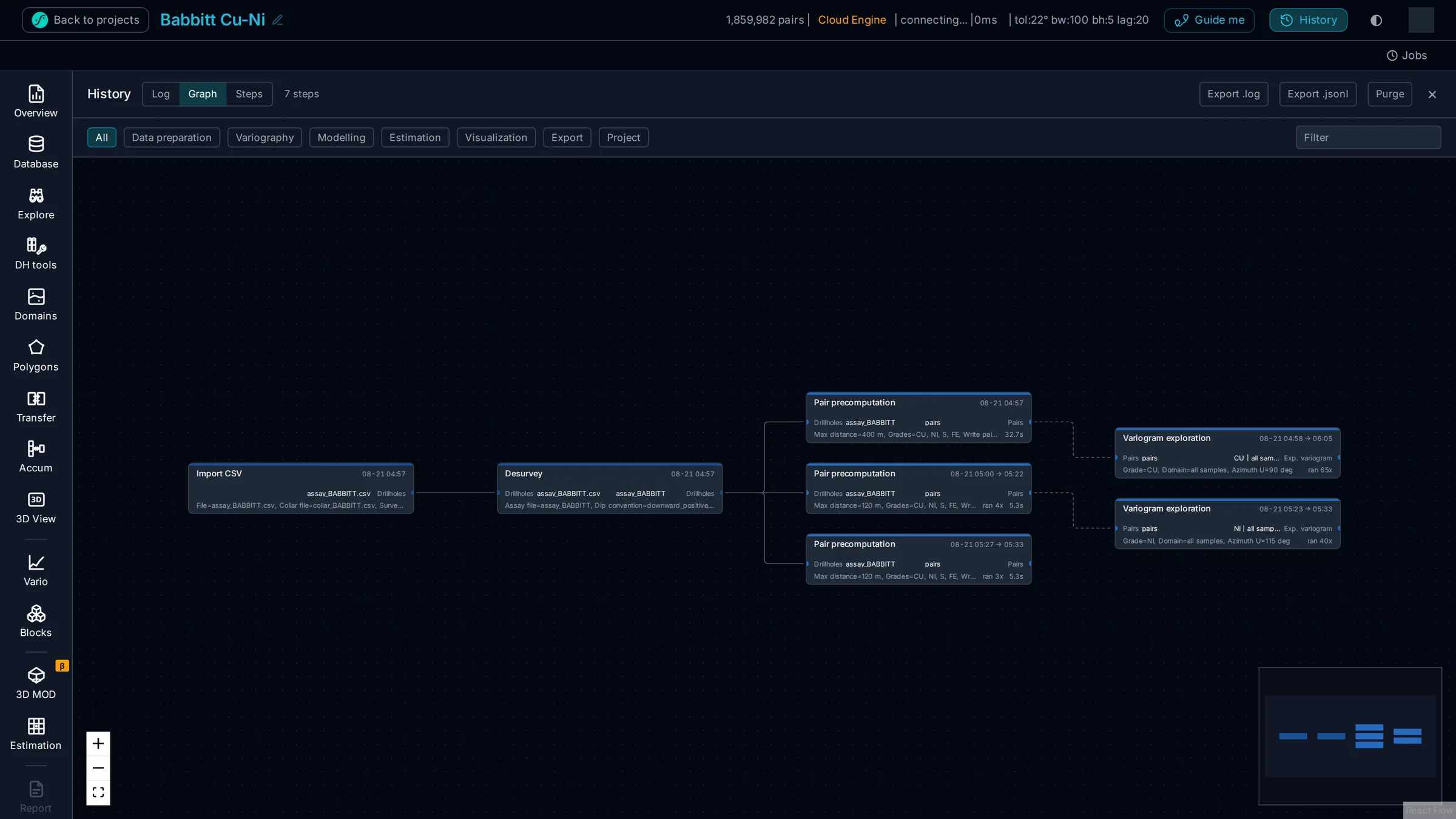
The licence you already pay for, driven by a routine your whole team can read.
Nobody has to learn the macro language to get the deliverable.
One source of truth
A model repository versions files. This versions the method. The drillholes, the composites, the domain rules, the fitted structures, the search ellipsoid and the routine that produced all of it sit in one project with one history. Nobody has to look in a folder, and nobody has to ask the person who ran it.
Which is what makes the audit quick. The week somebody normally spends rebuilding what was done — which file, which cut-off, which search, which version — is a week spent recovering a record that should have existed. Here it did exist, from the first import onward, and it exports in one action.
Onboarding
The reason people stay on the old software is rarely that it is better. It is that somebody spent two years learning it and nobody wants to spend two more. So the guide here runs inside the real product, on your own study, in chapters you choose — not a PDF, not a sandbox demo, not a two-day course somebody has to fly in for.
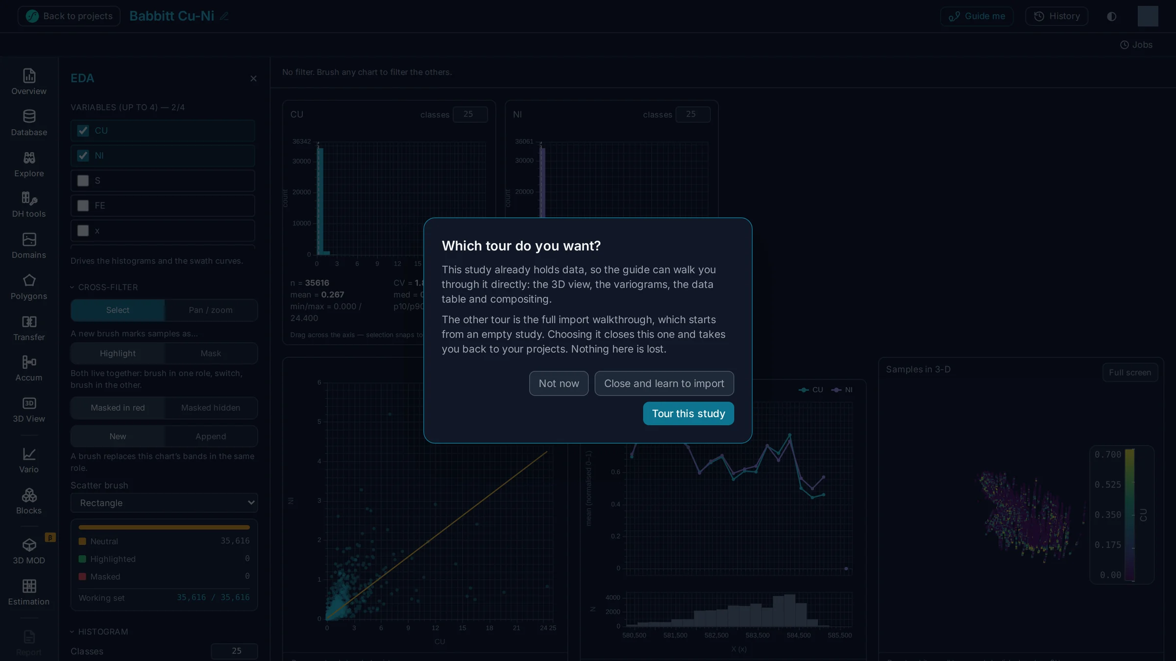
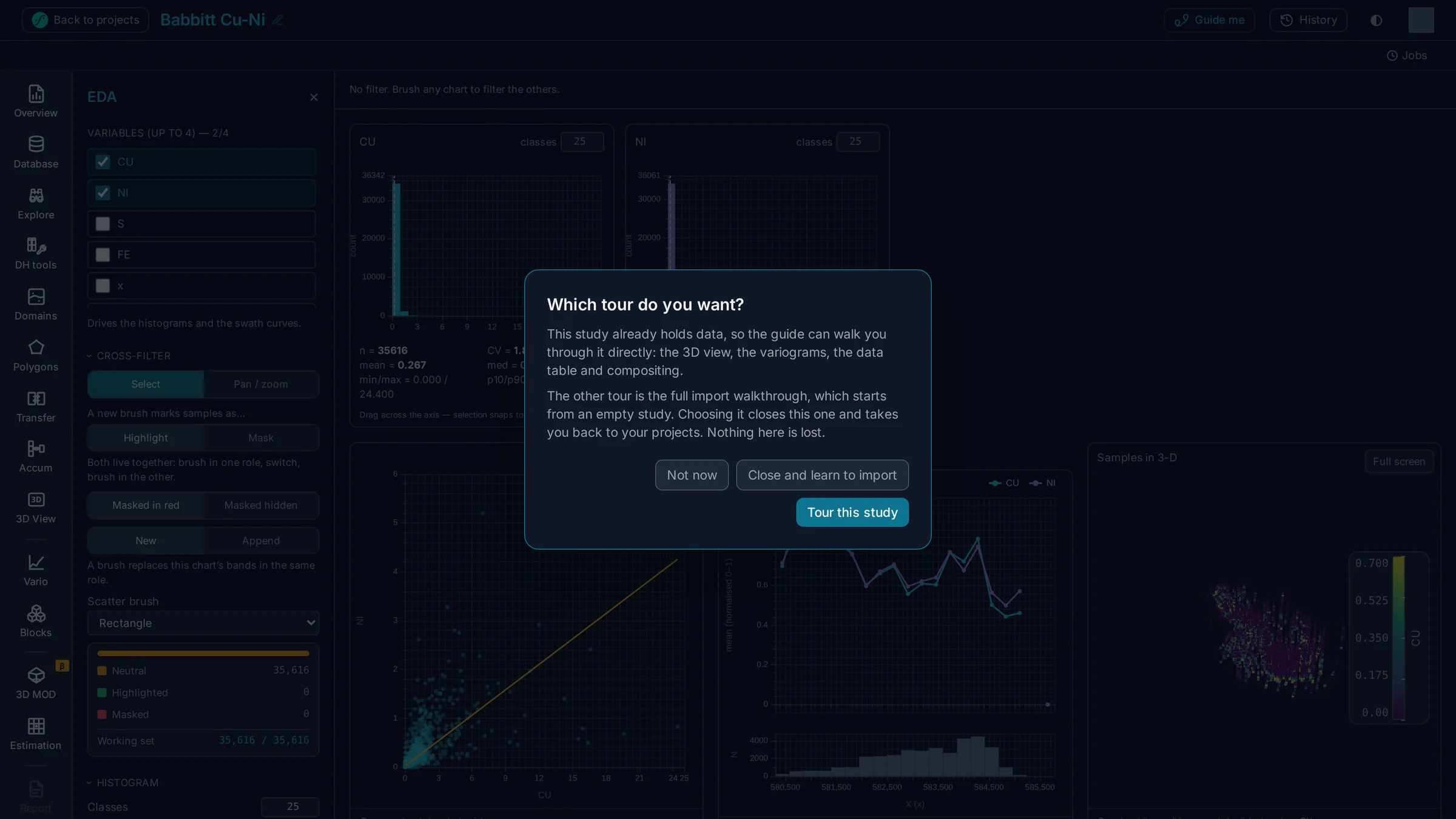
The tour walks the study you actually have — your 3D view, your variograms, your data table. A new geologist learns the deposit and the software in the same hour instead of transferring lessons from a fictional dataset afterwards.
The full path from an empty project through import and desurvey, or a short walk through the study in front of you. Nobody sits through the part they already know, which is the reason most in-app tours get dismissed on the first screen.
Walk the path once with your own conventions and your own domains, then send the team down the same one. Induction stops being a document somebody has to keep current and becomes the product itself.
Bring one dataset
Bring a collar / survey / assay trio from a deposit you know well. We load it in front of you, you take a direction off the variogram map yourself, and you see how long it takes to test the interpretation you have been putting off.
 beta
beta